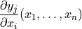
Automatic differentiation (AD)

Simply put, the aim of automatic differentiation (AD) is to automatically obtain the derivatives of somes variables output by an existing program with respect to some of its input variables.

It avoids resorting to symbolic differentiation, which is error-prone when done manually and quickly of excessive complexity when applied automatically, or finite differences, which are inexact.

To gain an intuition of the way this is achieved, consider a program computing return values of variables $y_j$ from values of arguments $x_i$ through intermediate values $v_k$ , where each value is obtained from its direct predecessors through elemental operations $(+, \times, /, \exp, \sf{etc.})$ .

Let us denote:

independent variables: $(x_i)_i, i \in \{1, 2, ..., n\}$ ,
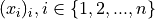dependent variables: $(y_j)_j, j \in \{1, 2, ..., m\}$ ,
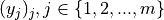intermediate values: $(v_k)_k$ which may or not be assigned to variables in the program,
relation: $i \prec j$ if $v_j$ depends on $v_i$ , eg. below $1 \prec 5$ .
predecessors: $u_j := (v_i)_{i \prec j}$ eg. below $u_5 = \begin{pmatrix} v_1 \\ v_2 \end{pmatrix}$
operation: $\varphi_j: u_j \mapsto v_j$ eg. below $v_5 = \varphi_5(u_5)$

Figure made with TikZ

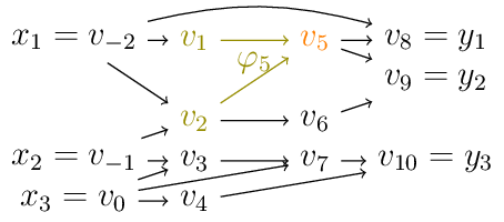
Example program

Since all programs can be reduced to sequential elemental operations in this fashion, automatic differentiation allows to compute $\dfrac{\partial y_j}{\partial x_i}(x_1, \ldots, x_n)$ by differentiating operations $\varphi_k : u_k \mapsto v_k$ and using the chain rule.

It comes in two main flavors, usually called forward- or tangent-mode and reverse- or adjoint-mode, which differ in the way substitutions are performed in the chain rule, which partial derivatives are computed as a result and the order in which statements in the original program are differentiated by the AD transformation.

Forward- or tangent-mode

Using the notations introduced above, forward-mode automatic differentiations allows to compute all derivatives w.r.t. a single independent variable $d \in (x_i)_i$ .

Let us denote the derivatives w.r.t. $d$ as

$\dot{v}_i = \dfrac{\partial v_i}{\partial d}$

such that the chain rule writes

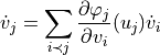
$\dot{v}_j = \sum_{i \prec j} \dfrac{\partial \varphi_j}{\partial v_i}(u_j) \dot{v}_i$

Forward-mode automatic differentation is equivalent to applying substitutions in the order indicated by the arrow in

$\dot{v}_{k+2} = \overleftarrow{\dfrac{\partial v_{k+2}}{\partial v_{k+1}} \underbrace{\left( \frac{\partial v_{k+1}}{\partial v_{k}} {\dot{v}_{k}} \right)}_{\dot{v}_{k+1}}}$

Initializing $\dot{d} = 1$ and $\dot{v}_k = 0, \forall v_k \neq d$ ,

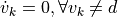we obtain in a single evaluation 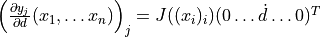$\left( \frac{\partial y_j}{\partial d}(x_1, \ldots x_n)\right)_j = J((x_i)_i) (0 \ldots \dot{d} \ldots 0)^T$

where $J$ is the Jacobian matrix $J = \nabla \begin{pmatrix} y_1(x_1, \ldots, x_n) \\ \vdots \\ y_m(x_1, \ldots, x_n) \end{pmatrix}$ .

Advantages and inconvenients

Forward-mode is easy to implement as derivatives can be computed in the same order of computation as that of the original program.

If there are less independent than dependent variables, its complexity is lower than that of the reverse- or adjoint-mode. But frequently, and maybe even more so in ocean and atmosphere models, the number of inputs greatly exceeds the number of outputs, requiring many repeated evaluations, one for each input or independent variable to differentiate with respect to.

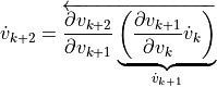
Reverse- or adjoint-mode

Using the notations introduced above, reverse-mode automatic differentiations allows to compute all derivatives of a single dependent variable $z \in (y_j)_j$ .

Let us denote the adjoints w.r.t. $z$ as

$\bar{v}_i = \dfrac{\partial z}{\partial v_i}$

such that the chain rule writes

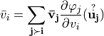
$\bar{v}_i = \sum_{\mathbf{{j \succ i}}} \mathbf{\bar{v}_j} \dfrac{\partial \varphi_j}{\partial v_i}(\mathbf{\overset{?}{u_j}})$

where bold font is used to highlight how the value of the adjoint $\bar{v}_i$ depends on successors of $v_i$ .

Reverse-mode automatic differentation is equivalent to applying substitutions in the order indicated by the arrow in

$\overrightarrow{\underbrace{\left( \bar{v}_{k} \dfrac{\partial v_{k}}{\partial v_{k-1}} \right)}_{\bar{v}_{k-1}} \dfrac{\partial v_{k-1}}{\partial v_{k-2}} } = \bar{v}_{k-2}$

Initializing $\bar{z} = 1$ and $\bar{v}_k = 0, \forall v_k \neq z$ ,

we obtain in a single evaluation $\left( \frac{\partial z}{\partial x_i}(x_1, \ldots, x_n)\right)_i = \nabla^T z(x_1, \ldots, x_n) = (0 \ldots \bar{z} \ldots 0) J(x_1, \ldots, x_n)$ .

Advantages and inconvenients

Reverse-mode is quite a lot more complicated to implement than forward-mode as adjoints need to be computed in the reversed order of computation compared to that of the original program as illustated in the example below.

If there are less dependent than independent variables, as is often the case, its complexity is lower than that of the forward- or tagent-mode.

However, when some variables are overwritten in the program, reverse-mode also requires running the original program and recording overwritten values, and eventually some the results of some operations, when they appear in the computations of some adjoints. This add further complications compared to forward-mode and requires using a persistent “tape”, which needs to be kept in memory, or recomputing values as many times as they are required.

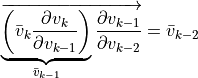
A simple example in reverse-mode with non-linearities

Let us consider the simple computations displayed below and illustate how to compute the adjoints $\bar{x}_1 = \dfrac{\partial z}{\partial x_1}$ and $\bar{x}_2 = \dfrac{\partial z}{\partial x_2}$ for a chosen dependent variable $z \in \{y_1, y_2\}$ .

Figure made with TikZ

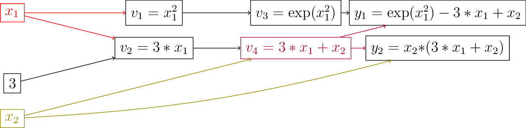
Simple program example

Figure made with TikZ

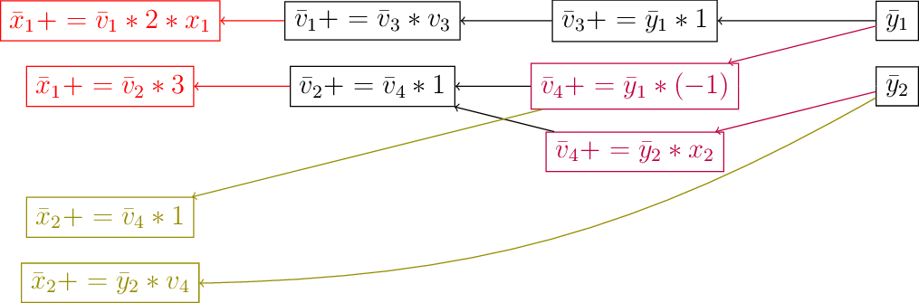
Reverse-mode example

Initialize with $\forall i, \bar{x}_i = 0, \forall k, \bar{v}_k = 0 \text{ and choose } (\bar{y}_1 = 1, \bar{y}_2 = 0) \text{ \textbf{or} } (\bar{y}_1 = 0, \bar{y}_2 = 1)$ to obtain the adjoints.

Notice that the adjoint of variables appearing as operands in the original computations (top) are incremented in the reverse-mode ones (bottom). Moreover, non-linearities in the original occasion the presence of operation results/ non-adjoint variables in the adjoint computations, which could be either recomputed or recorded and restored from a tape.